Post-acquisition technology integration simulator: the complete guide
This guide explains, with no prior knowledge assumed, a simulator that reproduces the integration of an acquired company: a team of 40 engineers migrates a platform over three years while keeping the existing service running. At the attrition observed in the reference case, the model produces no spiral of departures, even with the three protections removed. All numerical values in the model are synthetic. They serve to explore mechanisms and predict nothing.
Thierry Sayegh-Sauvage · updated 24 October 2026 · guide available in French and English
In brief
The simulator stages 40 engineers over 156 weeks. They must finish a migration and, at the same time, keep the existing platform running. Five ideas are enough to read everything else.
- An integration can run away through a chain of causes: departures reduce the team's capacity, the migration falls behind, uncertainty rises, and more people leave.
- The model contains three chains of this type and three protections: a retention bonus for key people, a rolling budget that funds replacements, and a parallel run of the old and the new system.
- At the attrition observed in the reference case (3 non-key departures over three years), the model produces no spiral, with or without the protections. The reference case therefore sat far from the tipping threshold.
- This result does not prove that the protections were useless. Without protection, half of the simulations tip into a spiral at about three times the observed attrition. With all three protections, it takes about ten times that attrition.
- All numerical values are synthetic. The model helps ask the right questions before signing an acquisition. It computes no forecast.
The problem: why an integration can run away
When a company buys another, two IT systems, two teams and two ways of working have to be brought together. Here, the engineering team of the acquired company must move its platform to a different technical infrastructure. That is the migration. Meanwhile, customers keep using the product, which means maintaining the existing service: fixing incidents, shipping small changes, keeping the service running. That is ongoing operations.
The weight of these operations depends on technical debt, meaning the accumulation of shortcuts taken in the past in code and infrastructure. The heavier the debt, the more engineers ongoing operations absorb. In the model, operations take 6% of engineering effort when debt is zero and 30% when debt is at its starting level. Less capacity remains for the migration and for paying down that same debt.
These mechanisms reinforce one another. Imagine a team that loses two people. The others take over their work, the migration slips, the announced schedule degrades, worry grows. Two more people leave in turn, and the cycle restarts faster. Specialists call this a reinforcing loop: the effect of each step feeds its own cause.
A spreadsheet represents this phenomenon poorly, because effects arrive with delays and depend on each individual. An agent-based simulator brings 40 individual engineers to life, each with a personal sensitivity to uncertainty, and lets the whole evolve week after week. One then observes whether the team holds or collapses, and what makes the difference.
The model at a glance
Each arrow links a cause to its effect. A plus means the two quantities move in the same direction, a minus that they move in opposite directions. The map merges migration progress and its delay into a single box. Dashed links exist in the model. The reference case showed no customer attrition: revenue exposure stayed theoretical there.
The model contains three reinforcing loops, chains of causes in which each effect feeds its own cause.
| Loop | Chain of causes | In plain terms |
|---|---|---|
| R1, attrition spiral | Departures, capacity, delay, uncertainty, departures | Departures slow the migration, which worries the teams and triggers more departures. |
| R2, debt and capacity | Debt, run load, capacity, debt | The heavier the debt, the less capacity the team has to reduce it. |
| R3, revenue pressure | Delay, revenue at risk, uncertainty, departures, capacity, delay | A delay threatens revenue, which worries the teams and sustains the delay. This loop stayed inactive in the reference case. |
The three levers slow these loops: the retention bonus acts on departures, the rolling budget on capacity, the parallel run on revenue at risk.
Variables and levers
The model tracks eight quantities that change every week, and three levers that can be switched on or off to measure their effect. All starting values are synthetic.
| Quantity | What it represents | Starting value |
|---|---|---|
| Engineering capacity | Sum of the productivities of the engineers present. A key person counts 1.5 times an ordinary person. A new hire climbs from 30% to 100% productivity over 16 weeks. | 40 people, including 8 key people |
| Run load | Share of capacity devoted to maintaining the existing service. It equals 6% plus 30% of the debt. | 30% |
| Technical debt | Level of accumulated shortcuts, from 0 to 1. It falls when the team pays it down and rises when delay pushes toward shortcuts. | 0.80 |
| Migration progress | Share of the total work already done, from 0 to 1. | 0 |
| Migration delay | Gap between the progress a linear plan over 156 weeks would have reached and the actual progress. | 0 |
| Revenue at risk | Customer revenue under threat as long as the migration is not finished: 15% of total revenue. Tracked revenue starts at 1 and can only fall. | 1 |
| Perceived uncertainty | Worry in the teams, from 0 to 1. It starts at the announcement of the integration, then evolves with delay, revenue pressure and recent departures. | 0.50 |
| Departures | Weekly probability of leaving the team, specific to each engineer: a base rate plus a reaction to uncertainty, weighted by personal sensitivity. | Value recalibrated on the observed case |
The three levers are the protections tested in the scenarios.
| Lever | What it does in the model |
|---|---|
| Retention bonus | Cuts the probability of departure of key people by 85% during the first 104 weeks. |
| Rolling budget | Each week, a three in ten chance of replacing a person who has left, as long as headcount is below 40. |
| Parallel run | Runs the old and the new system together. Costs 8% of capacity and protects 95% of revenue at risk against customer attrition. |
One week in the simulation
The program advances week by week. Each week, it performs the same eight calculations in the same order, then moves on to the next.
- Free capacity. The program adds up the productivity of the engineers present, then subtracts the run load and, if the parallel run is active, 8% of the starting capacity.
- Split. While the migration is unfinished, 25% of free capacity reduces the debt and 75% moves the migration forward. Once the migration is finished, all free capacity reduces the debt.
- Progress. Completed work is added to the total. Delay is the positive gap between the progress of a linear plan over 156 weeks and actual progress. In version 2, each departure adds rework to the total work.
- Debt. It falls with paydown effort and rises with delay, because a team that is behind takes shortcuts.
- Revenue. While the migration is unfinished, part of revenue is at risk. Without a parallel run, a delay loses customers. With it, 95% of that loss is avoided.
- Uncertainty. Each week it moves toward a target that adds up worry caused by the announcement (which fades with time), delay, revenue pressure and the departures of the last twelve weeks.
- Departures. Each engineer draws a random lot for leaving. The probability depends on the base rate, on uncertainty and on personal sensitivity. The retention bonus divides that probability by nearly seven for key people during 104 weeks. In version 2, a freelancer can only leave at the end of a contract.
- Arrivals. With the rolling budget, a person who has left is replaced with a three in ten chance each week, as long as headcount is below 40. The new hire reaches full productivity in 16 weeks.
A simulation repeats this cycle 156 times. The program then launches others, with different random draws, to see the spread of results.
The team: employees, freelancers and distance
The first version of the model treats all engineers as employees working in the same place, who can leave in any week. The reference case did not look like that: the team had a majority of freelancers, spread across locations. The second version adds these two traits and a third notion, knowledge loss, then compares three team structures.
| Characteristic | Co-located employees | Co-located freelancers | Distributed freelancers |
|---|---|---|---|
| Share of freelancers | 0% | 65% (assumption) | 65% (assumption) |
| When a departure is possible | Any week | At contract end, every 26 weeks for a freelancer | Same |
| Contracts with a common end date | Not applicable | 50% (assumption) | 50% (assumption) |
| Effort lost to coordination | 0% | 0% | 10% (assumption) |
| Ramp-up of a new hire | 16 weeks | 16 weeks | 24 weeks (assumption) |
| Contagion of departures between colleagues | Normal | Normal | Halved (assumption) |
Knowledge loss applies to all three structures. Each engineer accumulates knowledge of the migration during their first 52 weeks of presence, then nothing more is added. A key person carries three times as much. When someone leaves before the migration ends, the remaining work grows by a volume proportional to that knowledge: 20 person-weeks of rework per unit of knowledge.
The word “assumption” in the table flags unmeasured values. They influence the result and are listed with the others in the section on limits.
Calibrating: anchoring the model on the observed case
Calibrating means adjusting a model parameter until it reproduces an observed fact. The fact retained is the attrition of the reference case: about 3 non-key departures over the three years, in a team of around forty people. That statement allowed two readings. Reading A counts 3 departures in total over three years. Reading B counts 3 departures per year, 9 in total. The person who led the case confirmed reading A, which is the one used throughout this guide.
The method is a bisection search. One factor multiplies the base probability of departure and the reaction to uncertainty together, preserving their ratio. The program runs 50 to 60 simulations with a given factor, counts non-key departures, then narrows the factor until the average reaches 3. This gives the following values.
| Team structure | Factor | Base probability of departure per week | Reaction to uncertainty |
|---|---|---|---|
| Version 1, co-located employees | 0.1695 | 0.00034 | 0.00203 |
| Version 2, co-located employees | 0.1743 | 0.00035 | 0.00209 |
| Version 2, co-located freelancers | 0.1817 | 0.00036 | 0.00218 |
| Version 2, distributed freelancers | 0.1623 | 0.00032 | 0.00195 |
Two limits deserve attention before going further. First, the model has a single setting and a single observation: the agreement between the two holds by construction and tests nothing. Second, the split between the base rate and the reaction to uncertainty is an assumption that calibration cannot settle.
Results
Each scenario is simulated 40 to 60 times with different random draws. A simulation is classified as a “spiral” when engineering headcount falls below 60% of the initial headcount at any point. The tables give averages over these runs.
What a spiral looks like
The first figure shows the model with its default attrition, about 25 non-key departures over three years. This value was not recalibrated on the reference case: the figure shows the phenomenon without measuring it.
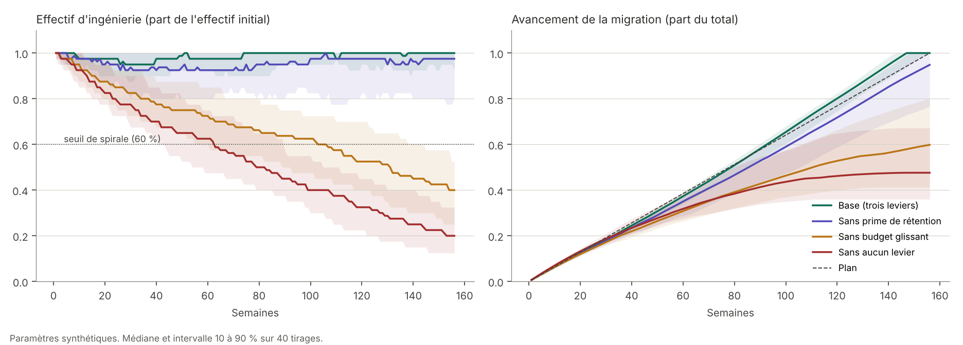
With all three levers, headcount stays close to its starting level (average minimum of 89%) and the migration finishes. Without the rolling budget, headcount falls on average to 40% and the migration stops at 60%. Without any lever, headcount reaches 21% and the migration plateaus at 50%. In this regime, 92% of the simulations without the rolling budget and 100% of the simulations without any lever tip into a spiral.
At the observed attrition
The following table uses version 2, the majority-freelance distributed team, recalibrated to 3 non-key departures over three years.
| Scenario | Spiral | Minimum headcount | Migration completed at 156 weeks | Final debt | Revenue lost | Key-person departures |
|---|---|---|---|---|---|---|
| Baseline, three levers | 0% | 97% | 94% | 0.25 | 0.7% | 0.3 |
| Without retention bonus | 0% | 97% | 92% | 0.26 | 0.7% | 0.8 |
| Without rolling budget | 0% | 91% | 88% | 0.30 | 0.8% | 0.5 |
| Without parallel run | 0% | 97% | 100% | 0.01 | 8.4% | 0.4 |
| Without any lever | 0% | 87% | 97% | 0.16 | 10.0% | 1.1 |
No scenario tips into a spiral. Each lever acts at a different point. The parallel run protects revenue: without it, 8.4% of revenue is lost against 0.7%. In return it costs capacity, hence a slower migration with it (94%) than without it (100%). The retention bonus retains key people: 0.3 departures on average with it, 0.8 without it.
Had the starting statement meant 3 departures per year, or 9 over three years (reading B), the result would differ. On the first version of the model, 35% of simulations without any lever would tip into a spiral, 8% without the rolling budget and none with all three levers.
What distance costs
| Team structure, baseline scenario | Migration completed at 156 weeks | Final debt | Revenue lost |
|---|---|---|---|
| Co-located employees | 100% | 0.00 | 0.4% |
| Co-located freelancers | 100% | 0.00 | 0.4% |
| Distributed freelancers | 94% | 0.25 | 0.7% |
Distance weighs on the schedule and on debt more than on the stability of the team. The 10% of effort lost to coordination and the 24 weeks of ramp-up are assumptions: this table describes their effect on the model and says nothing about the reality of the reference case.
Distance to the tipping threshold
The second figure answers the useful question: by how much would attrition have to rise for the system to tip? The horizontal axis multiplies the attrition calibrated on the observed case.
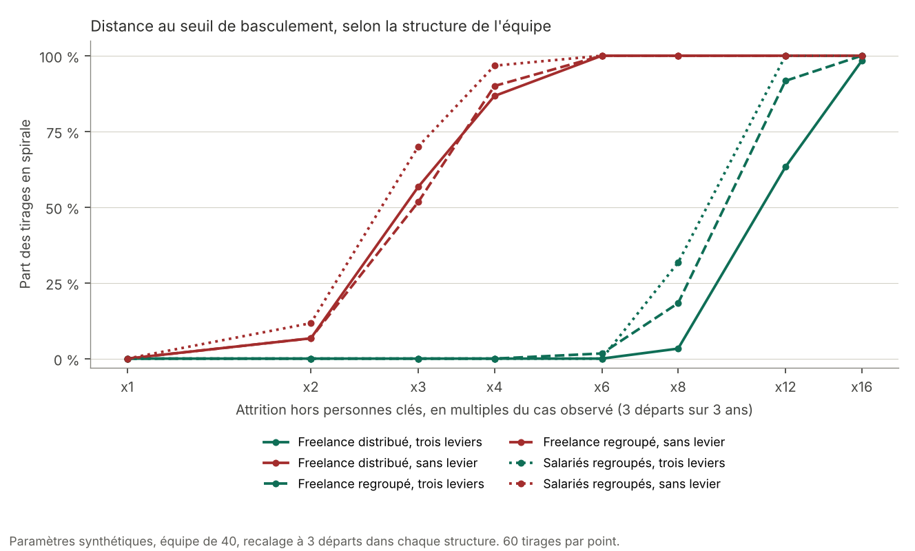
Without any lever, half of the simulations tip at about three times the observed attrition (57% for distributed freelancers, 52% for co-located freelancers, 70% for co-located employees). With all three levers, tipping occurs between eight and twelve times the observed attrition. The levers therefore push the threshold back by a factor of about three to four. The reference case sat at the far left of the figure, well away from the tipping zone.
How to read these results
Three readings are legitimate. Three others seem natural and are not.
What the results support.
- The spiral mechanism exists in the model: it appears as soon as attrition exceeds a threshold, and the levers push that threshold back.
- Each lever acts at a distinct point. The parallel run protects revenue, the rolling budget protects headcount, the retention bonus protects key people.
- The reference case, with 3 departures over three years, sits far from the threshold.
What the results do not support.
- That the protections were useless. Far from the threshold, they change nothing about stability. They keep their value as insurance against stronger attrition.
- That a distributed team of freelancers is more robust. This result follows from two assumptions: a departure possible only at contract end, and a contagion of departures halved by distance.
- That the model predicts a future integration. It compares scenarios on synthetic values and computes no real probability.
One last point of method: the reference case is a success. A model calibrated on a single success can display the right outcome without its mechanisms being exact. A failed integration case, even anonymised, would bring the missing information: it would allow the model to be tested on the other side of the threshold.
Limits and assumptions to verify
The table lists what is guessed or chosen without measurement. Each row gives the effect on the results and the check that would settle it.
| Assumption | Value used | Effect on the results | Check to perform |
|---|---|---|---|
| Share of freelancers | 65% | Sets the frequency of possible departures | Actual composition of the team |
| A freelancer leaves only at contract end | Every 26 weeks | If notice is short, departures become possible all year and the apparent robustness of the team drops | Notice periods and contract lengths |
| Contracts with a common end date | 50% | Concentrates possible departures on a few dates | Share of contracts renewed together |
| Effects of distance | 10% coordination loss, 24 weeks of ramp-up, contagion halved | Explain the remaining debt and the better resistance of the distributed team | Compare with the actual migration schedule |
| Split of capacity between migration and debt | 75% and 25% | Sets the speed of debt paydown | Trade-off actually made in practice |
| Key people | 20% of the team, productivity of 1.5, knowledge × 3 | Determines the value of the retention bonus | Who held the knowledge of the migration |
| Spiral threshold | Headcount below 60% of the start | Very strong ordinary attrition crosses the threshold with no loop at all: it measures attrition as much as the spiral | A definition based on the acceleration of departures |
| Split between base rate and reaction to uncertainty | Ratio preserved during calibration | Changes the relative weight of chance and contagion | A second set of observed departures |
| A single observed case | A success | Calibration tests nothing; a second lived case has not yet served as a test | A failed case, even anonymised |
Three scope notes complete the table. The simulated team has 40 people, like the reference case, and the model covers a single type of integration: the acquisition of a company by a group, with infrastructure migration and ongoing operations running in parallel. No internal company data is used, and the reference case is anonymised. The agents are explicit rules, deliberately: their behavior can be checked line by line.
Using the code
The code is written in Python with the Mesa library, designed for agent-based simulation. It was run with Python 3.13 and Mesa 3.5.1. The files go in a single folder, because some import others.
Source code and results: repository thierrysays/integration-attrition-simulator or archive integration-attrition-simulator-v1.1.zip (450 KB, Python scripts, results, figures, README in French and English). Code under the Apache License 2.0; results, figures and README under Creative Commons Attribution 4.0.
Installation
pip install mesa==3.5.1 matplotlibThe files
| File | Role |
|---|---|
pmi_model.py | Version 1 model: team of co-located employees |
run_scenarios.py | Lever-removal scenarios, sensitivity sweep, figure 1 |
calibrer_attrition.py | Calibration on 3 departures (readings A and B), distance to the threshold |
tracer_seuil.py | Tipping curve of version 1 |
pmi_model_v2.py | Version 2 model: freelancers, knowledge loss, distance |
run_v2.py | Calibration, scenarios and tipping curve of version 2, figure 2 |
redessiner_courbe_v2.py | Redraws figure 2 from the results file, without rerunning the simulations |
resultats_*.csv | Results tables, readable in a spreadsheet |
The commands
python3 run_scenarios.py
python3 calibrer_attrition.py
python3 run_v2.py
Each command prints its tables on screen and writes its results files to the folder. Duration was not measured precisely: allow a few minutes for the calibrations, which launch several hundred simulations.
Changing a value and rerunning
All model values are fields of a Params class. An example that rebuilds the distributed-freelancer team of version 2, with calibrated attrition, then runs one simulation without the retention bonus:
from dataclasses import replace
from pmi_model_v2 import IntegrationModel, Params

s = 0.1623  # facteur de calibrage, freelances distribués
p = replace(
    Params(),
    freelance_share=0.65, coordination_penalty=0.10,
    onboarding_weeks=24, w_dep=1.5,
    base_quit=0.002 * s, quit_gain=0.012 * s,
    retention_bonus=False,
)
resultat = IntegrationModel(p, seed=1).run().summary()
print(resultat)
The seed parameter fixes the random draws: the same value gives exactly the same result. The scripts use values from 1000 upward for scenarios, from 5000 upward for calibration.
Reading the results columns
| Column | Meaning |
|---|---|
spirale | Share of simulations whose headcount fell below 60% of the initial headcount |
eff_min | Lowest headcount reached, as a share of the initial headcount |
avancement | Share of the migration completed at 156 weeks |
dette | Final level of technical debt |
revenu_perdu | Share of revenue lost to customer attrition |
departs_cles, departs_autres | Average number of key-person departures and of other departures |
reprise | Share of migration work redone after departures (version 2) |
Glossary
| Term | Definition |
|---|---|
| Agent | A simulated element that decides according to rules. Here, an engineer. |
| Attrition | People leaving a team over a period. |
| Reinforcing loop | A chain of causes in which the final effect feeds the initial cause and amplifies the phenomenon. |
| Rolling budget | Continuously renewed funding that allows people who have left to be replaced. |
| Calibrate | Adjust a parameter so that the model reproduces an observed fact. |
| Technical debt | Shortcuts accumulated in code and infrastructure, which make every intervention heavier. |
| Full-time equivalent | Unit for measuring headcount: one full-time person equals one. Three full-time equivalents equal three people. |
| Ongoing operations | Work to keep the existing service running: incidents, fixes, small changes. |
| Parallel run | Running the old and the new system at the same time, to avoid any interruption for customers. |
| Freelancer | Independent engineer bound by a fixed-term contract. |
| Random seed | A number that fixes the random draws. The same seed gives the same result. |
| Lever | A protection that can be switched on or off in a scenario. |
| Migration | Moving the platform to a different technical infrastructure. |
| Knowledge loss | Knowledge of the migration that leaves with a person and is paid for in rework. |
| Key person | An engineer who is more productive and carries more knowledge. 20% of the team in the model. |
| Retention bonus | A bonus paid to key people to keep them until the end of a period. |
| Rework | Work already done that must be redone or relearned after a departure. |
| Revenue at risk | Share of customer revenue under threat as long as the migration is not finished. |
| Sensitivity to uncertainty | Each engineer's own propensity to leave when worry rises. |
| Tipping threshold | Level of attrition beyond which simulations go into a spiral. |
| Agent-based simulation | A method that brings simulated individuals to life and observes what emerges from their interactions. |
| Spiral | In this guide, a simulation whose headcount falls below 60% of the initial headcount. |
| Synthetic | A value invented to illustrate a mechanism, not measured on a real case. |
| Run | One execution of the simulation with its own random draws. Each scenario has 40 to 60. |
Open questions and next steps
Four pieces of information remain to be gathered. Each settles one assumption of the limits table.
- What notice period and contract length did the freelancers have?
- Did the migration meet the three-year schedule? The answer sets the effort lost to coordination.
- What share of freelance contracts had a common end date?
- Is there a failed integration case, even anonymised, to test the model on the other side of the threshold?
The next steps, in order:
- Replace the contract-end constraint for freelancers with a departure possible at any time after notice, then rerun the tipping curve.
- Define the spiral by the acceleration of departures rather than by the final level of headcount.
- Test a second integration case without readjusting the parameters, then confront the model with a failed case.
- Submit the causal map and the assumptions to two people who have lived through an integration.
- Build a set of anonymised cases: this is the lasting asset of the project, far more than the code.
The values in this guide are synthetic and the reference case is anonymised. To discuss the model or submit an anonymised integration case, write to thierry@glossolalie.pro · linkedin.com/in/thierrys.